Overview

cerebroApp v1.3 provides new possibilities to export and visualize custom data that you would like to share alongside with your scRNA-seq data. At the time of writing, you can attach tables and plots (made with ggplot2) to your data set. In this article, I will show you to do it.

Tables

In previous cerebroApp versions, a very specific format for tables containing marker genes and enriched pathways was expected, resulting in a severe limitation of which methods you can use to generate the results, or alternatively requiring manual modification of the table to fit the format. Since cerebroApp v1.3, it is possible to export and visualize tables of any format in Cerebro, as long as they are a data.frame. Due to dynamic column formatting and color highlighting, the table content can be visually enhanced anyway.

Marker genes and enriched pathways

Let’s assume you have a Seurat object but generated tables of differentially expressed genes and enriched pathways using other tools/methods than those built into cerebroApp. To export those tables, you just need to put it in the right place, following a “method” and “name” scheme. In this example, we assume you have a table of marker genes called custom_table that looks like this:

library(tibble)

custom_table <- tribble(
      ~a,   ~b,  ~c,       ~d,      ~e,
  "this", "is", "a", "custom", "table"
)

To make sure it is exported when running exportFromSeurat(), simply save it in a list with a name for both the method and the table, e.g. custom_method and custom_table:

pbmc_Seurat@misc$marker_genes[['custom_method']] <- list(
  "custom_table" = custom_table
)

Then, you can export your data set:

exportFromSeurat(
  pbmc_Seurat,
  assay = 'SCT',
  slot = 'data',
  file = '~/Dropbox/Cerebro_development/pbmc_Seurat.crb',
  experiment_name = 'pbmc_Seurat',
  organism = 'hg',
  groups = c('sample','seurat_clusters','cell_type_singler_blueprintencode_main'),
  cell_cycle = c('cell_cycle_seurat'),
  nUMI = 'nCount_RNA',
  nGene = 'nFeature_RNA',
  add_all_meta_data = TRUE,
  verbose = FALSE
)

[15:28:21] Start collecting data...
[15:28:21] Overview of Cerebro object:

class: Cerebro_v1.3
cerebroApp version: 1.3.0
experiment name: pbmc_Seurat
organism: hg
date of analysis: 2020-02-19
date of export: 2020-09-10
number of cells: 5,697
number of genes: 15,907
grouping variables (3): sample, seurat_clusters, cell_type_singler_blueprintencode_main
cell cycle variables (1): cell_cycle_seurat
projections (2): UMAP, UMAP_3D
trees (3): sample, seurat_clusters, cell_type_singler_blueprintencode_main
most expressed genes: sample, seurat_clusters, cell_type_singler_blueprintencode_main
marker genes:
 - cerebro_seurat (3): sample, seurat_clusters, cell_type_singler_blueprintencode_main, 
 - custom_method (1): custom_table
enriched pathways:
 - cerebro_seurat_enrichr (3): sample, seurat_clusters, cell_type_singler_blueprintencode_main, 
 - cerebro_GSVA (3): sample, seurat_clusters, cell_type_singler_blueprintencode_main
trajectories:
 - monocle2 (1): highly_variable_genes

[15:28:21] Saving Cerebro object to: ~/Dropbox/Cerebro_development/pbmc_Seurat.crb
[15:28:27] Done!

You can see that among the marker gene results is the custom_method and custom_table.

Then, after loading the data into Cerebro, we will see this:

Granted, this isn’t a very pretty table, but you get the idea.

Extra material

When you have tables that might be useful to interpret the data set but don’t contain marker genes, differentially expressed genes, or enriched pathways, then you can add them as extra material. Again, just make sure you follow the general structure. In the case of a Seurat object, store the tables with an interpretable name in a list at @misc$extra_material$tables. You can see an example below, where we store the same example table as before:

custom_table <- tibble(
  a = "this",
  b = "is",
  c = "a",
  d = "test"
)

pbmc_Seurat@misc$extra_material$tables <- list(
  "test" = custom_table
)

exportFromSeurat(
  pbmc_Seurat,
  assay = 'SCT',
  slot = 'data',
  file = '~/Dropbox/Cerebro_development/pbmc_Seurat.crb',
  experiment_name = 'pbmc_Seurat',
  organism = 'hg',
  groups = c('sample','seurat_clusters','cell_type_singler_blueprintencode_main'),
  cell_cycle = c('cell_cycle_seurat'),
  nUMI = 'nCount_RNA',
  nGene = 'nFeature_RNA',
  add_all_meta_data = TRUE,
  verbose = FALSE
)

[15:07:48] Start collecting data...
[15:07:50] Overview of Cerebro object:

class: Cerebro_v1.3
cerebroApp version: 1.3.0
experiment name: pbmc_Seurat
organism: hg
date of analysis: 2020-02-19
date of export: 2020-09-11
number of cells: 5,697
number of genes: 15,907
grouping variables (3): sample, seurat_clusters, cell_type_singler_blueprintencode_main
cell cycle variables (1): cell_cycle_seurat
projections (2): UMAP, UMAP_3D
trees (3): sample, seurat_clusters, cell_type_singler_blueprintencode_main
most expressed genes: sample, seurat_clusters, cell_type_singler_blueprintencode_main
marker genes:
  - cerebro_seurat (3): sample, seurat_clusters, cell_type_singler_blueprintencode_main, 
  - custom_method (1): custom_table
enriched pathways:
  - cerebro_seurat_enrichr (3): sample, seurat_clusters, cell_type_singler_blueprintencode_main, 
  - cerebro_GSVA (3): sample, seurat_clusters, cell_type_singler_blueprintencode_main
trajectories:
  - monocle2 (1): highly_variable_genes
extra material:
  - tables (1): test

[15:07:50] Saving Cerebro object to: ~/Dropbox/Cerebro_development/pbmc_Seurat.crb
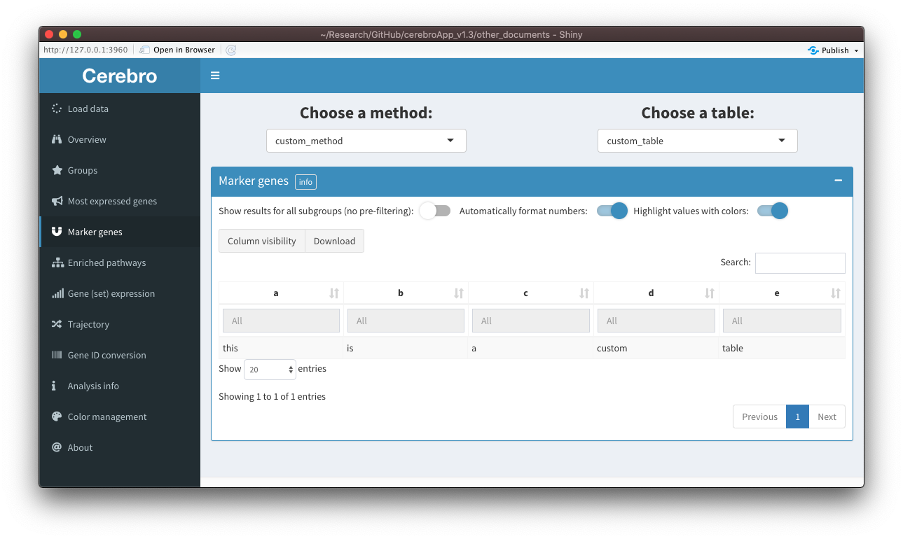
[15:07:55] Done!

This time, you see that our table with the name “test” was exported as part of the extra material. In Cerebro, when a data set contains extra material, a tab will appear in the side bar which will give you access to the table, as shown in the screenshot:

Again, this table isn’t particularly informative, but hopefully you got an idea of the procedure.

Plots

Custom plots can be exported and visualized in the “Extra material” tab as well. The only requirement is that they were produced with ggplot2. You can switch between an interactive version of the plot (converted with plotly) or the unmodified plot.

Example #1

Let’s look at an example in which we create a simple plot with ggplot2, call it iris, and add it to the Seurat object:

library(ggplot2)

custom_plot <- ggplot(iris, aes(Sepal.Length, Sepal.Width, color = Species)) +
  geom_point()

pbmc_Seurat@misc$extra_material$plots <- list(
  "iris" = custom_plot
)

exportFromSeurat(
  pbmc_Seurat,
  assay = 'SCT',
  slot = 'data',
  file = '~/Dropbox/Cerebro_development/pbmc_Seurat.crb',
  experiment_name = 'pbmc_Seurat',
  organism = 'hg',
  groups = c('sample','seurat_clusters','cell_type_singler_blueprintencode_main'),
  cell_cycle = c('cell_cycle_seurat'),
  nUMI = 'nCount_RNA',
  nGene = 'nFeature_RNA',
  add_all_meta_data = TRUE,
  verbose = FALSE
)

[11:54:33] Start collecting data...
[11:54:33] Overview of Cerebro object:

class: Cerebro_v1.3
cerebroApp version: 1.3.0
experiment name: pbmc_Seurat
organism: hg
date of analysis: 2020-02-19
date of export: 2020-09-24
number of cells: 5,697
number of genes: 15,907
grouping variables (3): sample, seurat_clusters, cell_type_singler_blueprintencode_main
cell cycle variables (1): cell_cycle_seurat
projections (2): UMAP, UMAP_3D
trees (3): sample, seurat_clusters, cell_type_singler_blueprintencode_main
most expressed genes: sample, seurat_clusters, cell_type_singler_blueprintencode_main
marker genes:
  - cerebro_seurat (3): sample, seurat_clusters, cell_type_singler_blueprintencode_main
enriched pathways:
  - cerebro_seurat_enrichr (3): sample, seurat_clusters, cell_type_singler_blueprintencode_main, 
  - cerebro_GSVA (3): sample, seurat_clusters, cell_type_singler_blueprintencode_main
trajectories:
  - monocle2 (1): highly_variable_genes
extra material:
  - plots (1): iris

[11:54:33] Saving Cerebro object to: ~/Dropbox/Cerebro_development/pbmc_Seurat_dgCMatrix.crb
[11:54:37] Done!

In the log messages of the export process, we see that the plot was correctly extracted and is listed in the “extra material”.

In Cerebro, we can now access this table in the “Extra material” tab through the “plots” category.

Example #2

In the second example, we prepare a dot plot showing the expression of the most significant marker gene for each cluster.

library(dplyr)
library(ggplot2)
library(tidyr)

# cells will be grouped by clusters that they have been assigned to
cluster_ids <- levels(seurat@meta.data$seurat_clusters)

# select a set of genes for which we want to show expression
genes_to_show <- seurat@misc$marker_genes$cerebro_seurat$seurat_clusters %>%
  group_by(seurat_clusters) %>%
  arrange(p_val_adj) %>%
  slice(1) %>%
  pull(gene)

# for every cluster-gene combination, calculate the average expression across
# all cells and then transform the data into a data frame
expression_levels_per_cluster <- vapply(
    cluster_ids, FUN.VALUE = numeric(length(cluster_ids)), function(x) {
      cells_in_current_cluster <- which(seurat@meta.data$seurat_cluster == x)
      Matrix::rowMeans(seurat@assays$SCT@data[genes_to_show,cells_in_current_cluster])
    }
  ) %>%
  t() %>%
  as.data.frame() %>%
  mutate(cluster = rownames(.)) %>%
  select(cluster, everything()) %>%
  pivot_longer(
    cols = c(2:ncol(.)),
    names_to = 'gene'
  ) %>%
  rename(expression = value) %>%
  mutate(id_to_merge = paste0(cluster, '_', gene))

# for every cluster-gene combination, calculate the percentage of cells in the
# respective group that has at least 1 transcript (this means we consider it
# as expressing the gene) and then transform the data into a data frame
percentage_of_cells_expressing_gene <- vapply(
    cluster_ids, FUN.VALUE = numeric(length(cluster_ids)), function(x) {
      cells_in_current_cluster <- which(seurat@meta.data$seurat_cluster == x)
      Matrix::rowSums(seurat@assays$SCT@data[genes_to_show,cells_in_current_cluster] != 0)
    }
  ) %>%
  t() %>%
  as.data.frame() %>%
  mutate(cluster = rownames(.)) %>%
  select(cluster, everything()) %>%
  pivot_longer(
    cols = c(2:ncol(.)),
    names_to = 'gene'
  ) %>%
  rename(cell_count = value) %>%
  left_join(
    .,
    seurat@meta.data %>%
      group_by(seurat_clusters) %>%
      tally() %>%
      rename(cluster = seurat_clusters),
    by = 'cluster') %>%
  mutate(
    id_to_merge = paste0(cluster, '_', gene),
    percent_cells = cell_count / n
  )

# merge the two data frames created before and plot the data
custom_plot <- left_join(
    expression_levels_per_cluster,
    percentage_of_cells_expressing_gene %>% select(id_to_merge, percent_cells),
    by = 'id_to_merge'
  ) %>%
  mutate(
    cluster = factor(cluster, levels = rev(cluster_ids)),
    gene = factor(gene, levels = genes_to_show)
  ) %>%
  ggplot(aes(gene, cluster)) +
  geom_point(aes(color = expression, size = percent_cells)) +
  scale_color_distiller(
    palette = 'Reds',
    direction = 1,
    name = 'Log-normalised\nexpression',
    guide = guide_colorbar(frame.colour = "black", ticks.colour = "black")
  ) +
  scale_size(name = 'Percent\nof cells', labels = scales::percent) +
  labs(y = 'Cluster', color = 'Expression') +
  coord_fixed() +
  theme_bw() +
  theme(
    axis.title.x = element_blank(),
    axis.text.x = element_text(angle = 45, hjust = 1)
  )

With the plot ready, we can store it in the Seurat object and export it as before.

seurat@misc$extra_material$plots <- list(
  "dot_plot_marker_genes_clusters" = custom_plot
)

exportFromSeurat(
  seurat,
  assay = 'SCT',
  slot = 'data',
  file = '~/Dropbox/Cerebro_development/pbmc_Seurat.crb',
  experiment_name = 'pbmc_Seurat',
  organism = 'hg',
  groups = c('sample','seurat_clusters','cell_type_singler_blueprintencode_main'),
  cell_cycle = c('cell_cycle_seurat'),
  nUMI = 'nCount_RNA',
  nGene = 'nFeature_RNA',
  add_all_meta_data = TRUE,
  verbose = FALSE
)

[10:03:13] Start collecting data...
[10:03:14] Overview of Cerebro object:

class: Cerebro_v1.3
cerebroApp version: 1.3.0
experiment name: pbmc_Seurat
organism: hg
date of analysis: 2020-02-19
date of export: 2020-09-25
number of cells: 5,697
number of genes: 15,907
grouping variables (3): sample, seurat_clusters, cell_type_singler_blueprintencode_main
cell cycle variables (1): cell_cycle_seurat
projections (2): UMAP, UMAP_3D
trees (3): sample, seurat_clusters, cell_type_singler_blueprintencode_main
most expressed genes: sample, seurat_clusters, cell_type_singler_blueprintencode_main
marker genes:
  - cerebro_seurat (3): sample, seurat_clusters, cell_type_singler_blueprintencode_main
enriched pathways:
  - cerebro_seurat_enrichr (3): sample, seurat_clusters, cell_type_singler_blueprintencode_main, 
  - cerebro_GSVA (3): sample, seurat_clusters, cell_type_singler_blueprintencode_main
trajectories:
  - monocle2 (1): highly_variable_genes
extra material:
  - plots (1): dot_plot_marker_genes_clusters

[10:03:14] Saving Cerebro object to: ~/Dropbox/Cerebro_development/pbmc_Seurat.crb
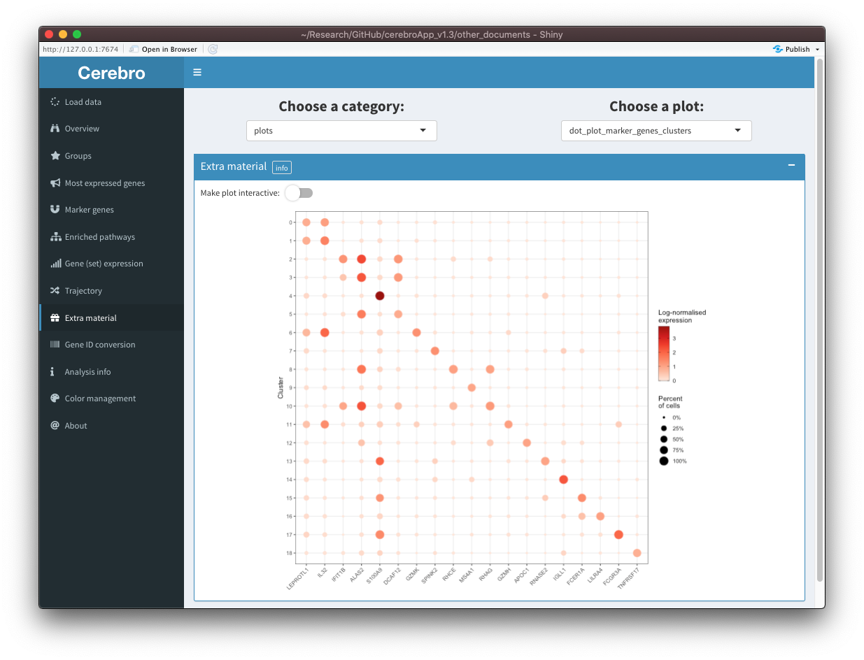
[10:03:18] Done!

Shown in the first screenshot is the interactive version of the plot:

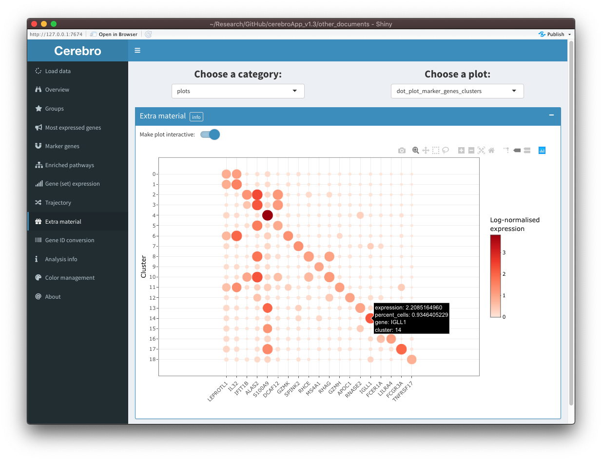
We notice that the legend for the dot size is missing. In cases where the plot isn’t shown correctly (conversion with plotly works well but not always perfectly), you can switch of interactivity and see the plain, unmodified plot:

Export and visualize custom tables and plots

Roman Hillje