Introduction to the Cerebro interface (v1.2 and older)

Roman Hillje

12 March, 2021

Introduction to Cerebro

This article is meant to give an introduction to Cerebro for people who don’t have any bioinformatic skills. Maybe you are an experimental biologists who performed a scRNA-seq experiment and the computational biologists who analysed the data for you gave you a file and told you to load it into Cerebro. And, maybe, he/she didn’t tell you what Cerebro is and what it can be used for. If this sounds like you, then this article should bring you up to speed.

To get yourself familiar with Cerebro, you don’t need a real data file yet. The application comes with a small data set pre-loaded which will allow you to get an idea of what Cerebro will show you about your own data. If you prefer a more authentic feeling, you can also download one of the example data sets we have prepared for illustrative purposes.

What you need

You need two things to start exploring your data:

1. The Cerebro application. The easiest way to get Cerebro is to download the standalone executable for either Windows or macOS (whichever operating system you are using) from the Cerebro releases. After the download is finished, the application can be unzipped and launched.
2. A file containing your data. This is the file you get from your colleague who did the analysis (the file name should end with .crb or .rds).

The interface

After launching Cerebro, you will see the Cerebro dashboard with all available panels on the left. We will go through each panel and see what information is be available there.

A few general notes:

• Please note that we have placed “info” boxes in many title bars which might provide helpful information.
• Most plots are interactive. Hover over them with your cursor to get additional information.
• Plots can be exported either to a PDF file (dimensional reductions; dedicated button in the title bar) or to a file PNG file (a small button in the top right corner of the plot that looks like a camera).
• Tables can be sorted (by clicking on the respective column title). Some can also be searched through the respective search boxes, and exported to either CSV or Excel format. Those tables which can be exported also have a “Column visibility” button which allows to hide some columns (which is useful on small screens and/or when there are many columns). Please note that in some tables some columns are hidden by default and need to be activated to be seen.

Load data

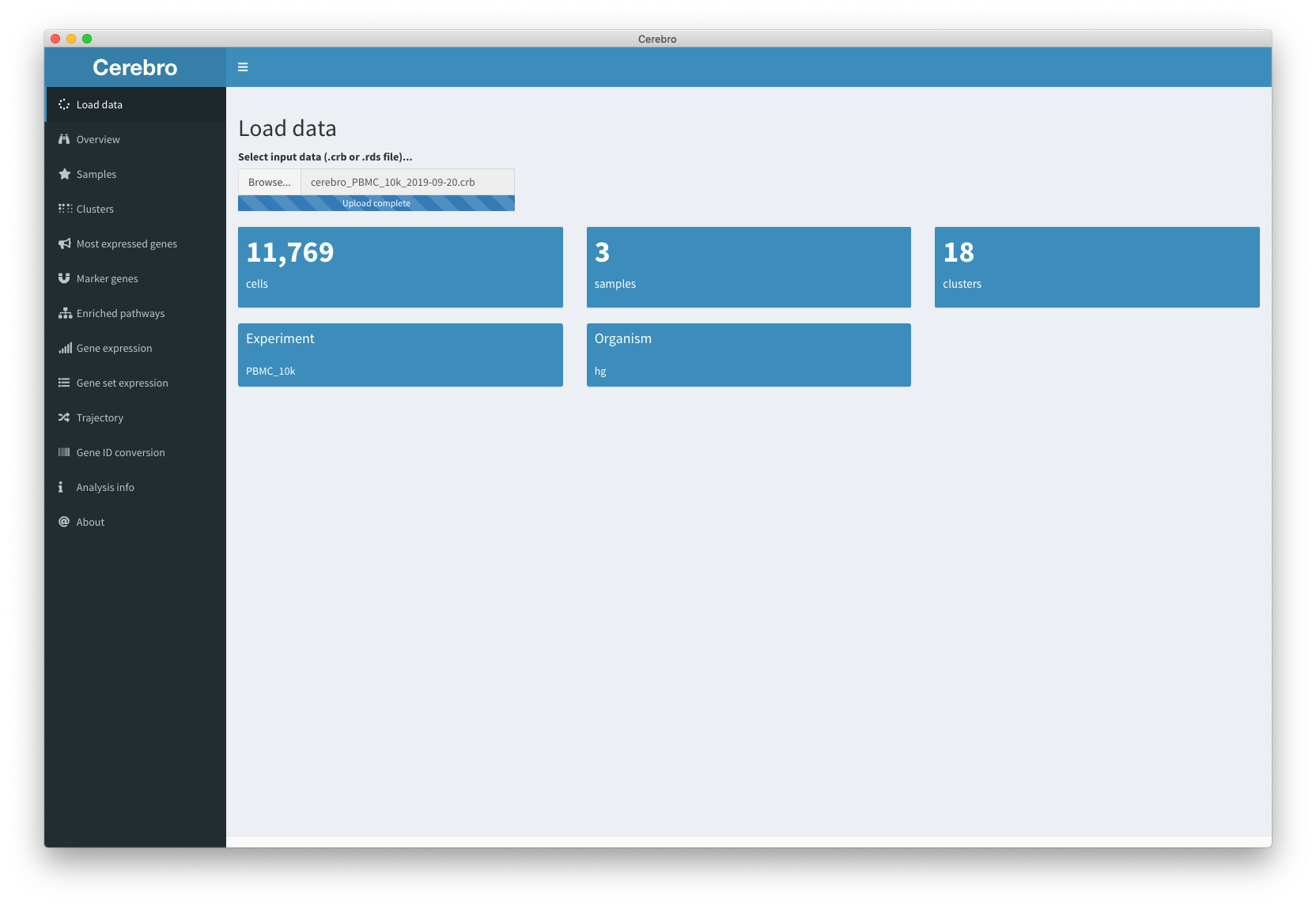
This is the panel that we will be shown to you when you launch Cerebro. In the top input panel you can choose your data which is the file you received from your colleague or downloaded from the examples mentioned earlier. The input file usually has the .crb or .rds extension. After selecting the file in the dialog box, the file will be loaded. Please be patient during this process and wait until the progress bar says “Upload complete.”. The numbers in the different tiles will now update and give you some numbers about your data sets, including the number of cells, number of samples, number of clusters, the organism, and the experiment name. After loading the sample, there is not much more to do here so let’s move on to the “Overview” panel.

Overview

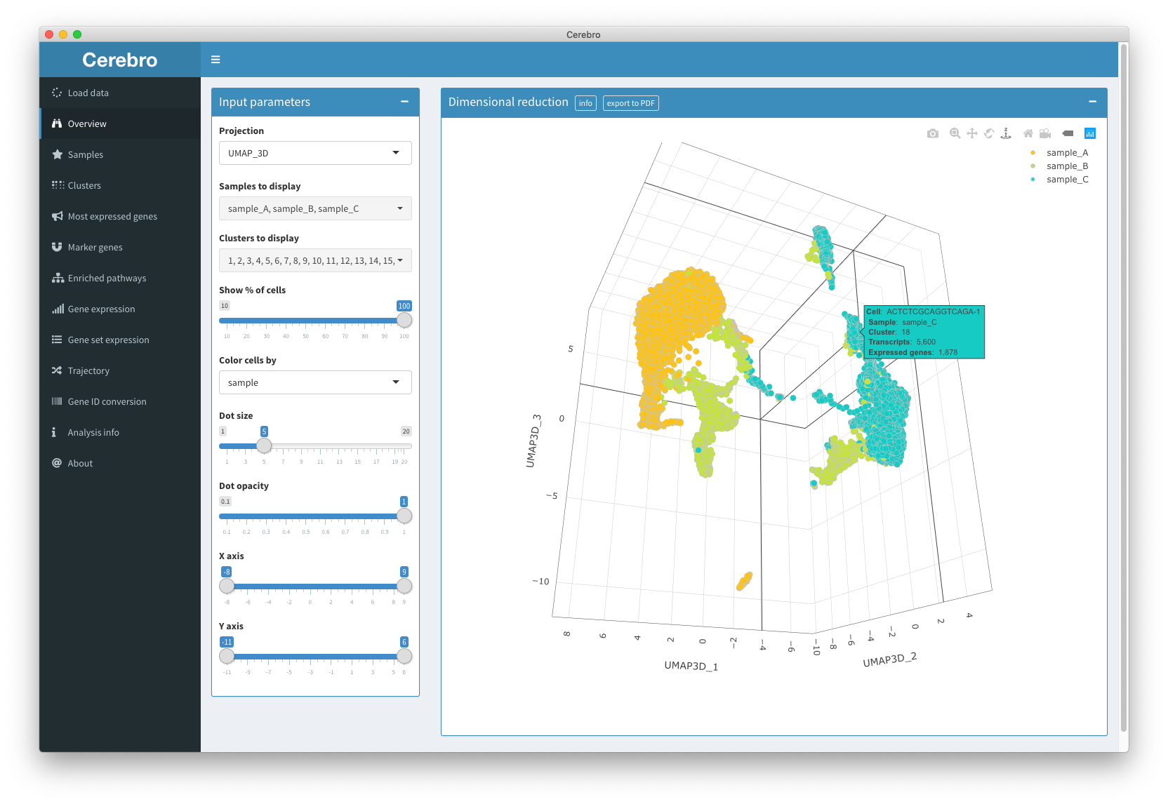
In the “Overview” panel, you have access to all the dimensional reductions (e.g. t-SNE or UMAP) that have been generated for this data set. Dimensional reductions can be either 2- or 3-dimensional and aim to represent the complex expression profiles of all the cells in a more interpretable way.

The plot is interactive which means you can hover over the cells with your cursor to get extra info, zoom in and out, and pan around. You may also export the plot to a PDF image by hitting the “export to PDF” button in the title bar. The file will the stored on your desktop.

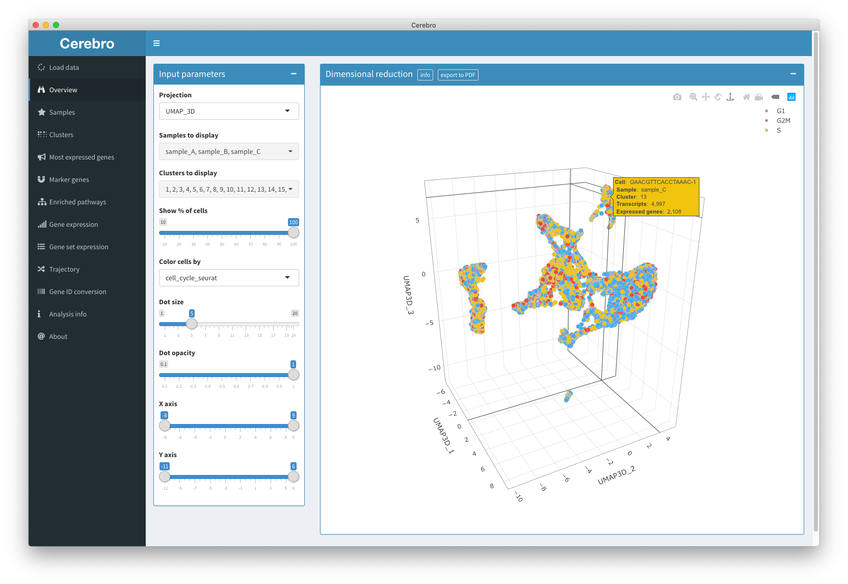
In the input box on the left, you can select a bunch of parameters for the plot. For example, if there are multiple dimensional reductions, you can choose which one should be shown. Also, you can exclude entire samples or clusters from the plot. Sometimes, data sets can become quite large which can make the plots dreadfully slow on older machines. In those cases, consider showing only a random subset of cells by dragging the slider down from 100% to a lower value. Next, you can choose which meta information to color the cells by. By default, they will be colored by the sample the cells originate from, but you can change this to any meta information that is available, e.g. cluster label, cell cycle phase, etc. The rest of the parameters are aesthetic and allow you to adjust dot size, dot opacity (transparency), and range of the X and Y scale.

Samples

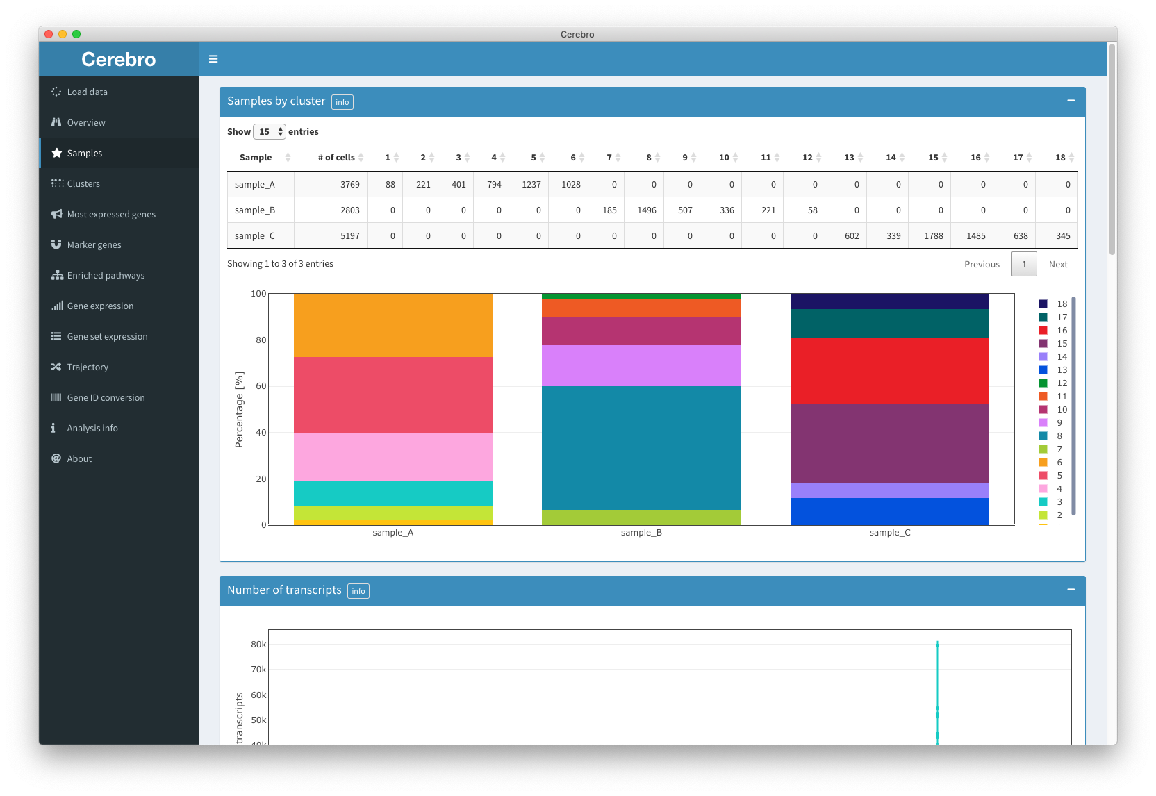
The “Samples” panel gives you a sample-centric view of the loaded data. That means, cells are grouped by the sample they came from.

First, you’ll see a table and bar plot showing you the composition of samples by the identified cluster.

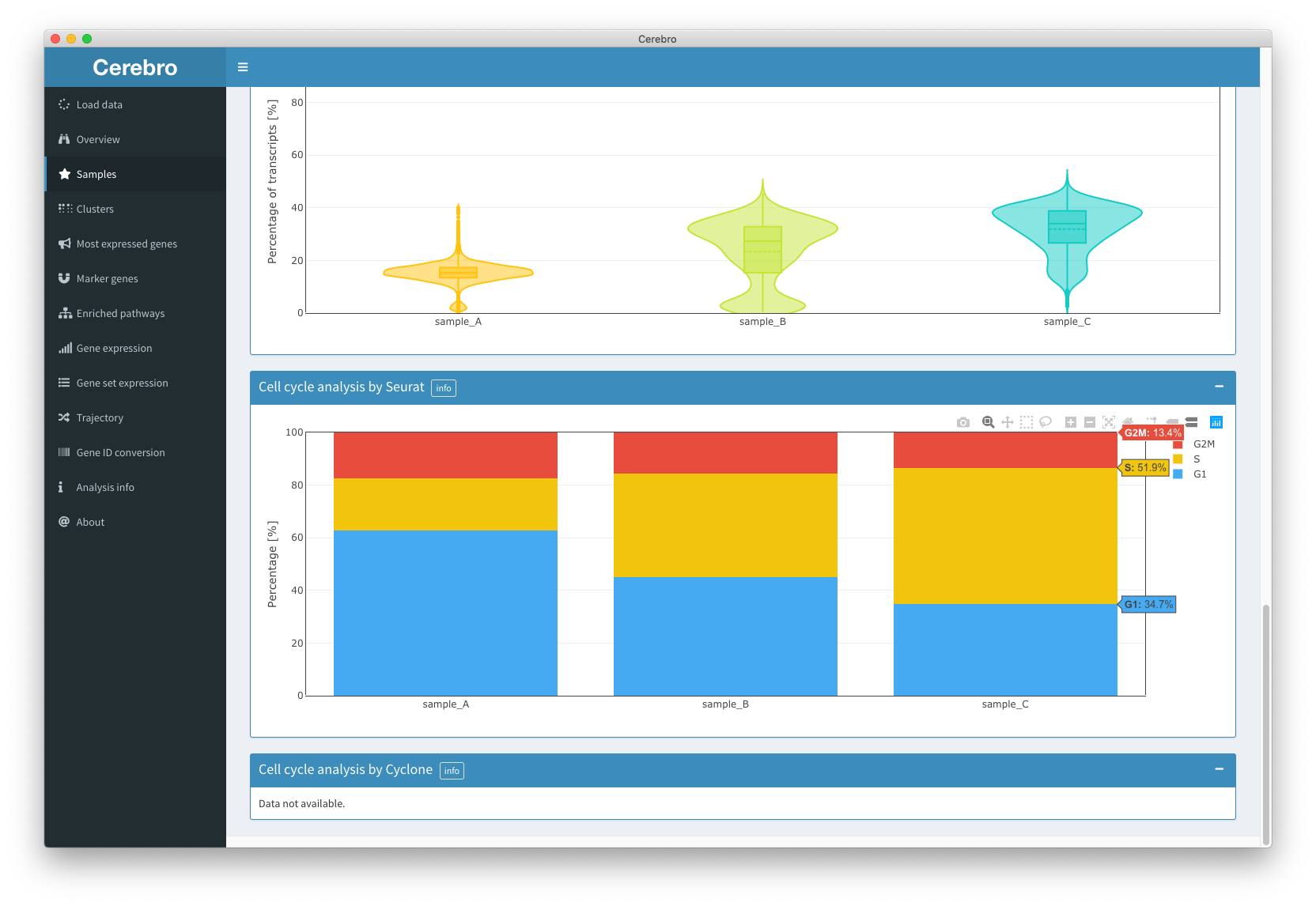
Then, you will see the distribution of the number of transcripts by sample in the form of a violin plot. More statistical info, such as the mean, median, quartiles, and min/max values, is shown when hovering over the distributions.

The same violin + box plot format is then used to show you the distribution of the number of expressed genes per sample, and, if available, also of the percentage of mitochondrial and ribosomal genes (percentage of transcripts coming from mitochondrial/ribosomal genes).

The last two boxes, if available, show the percentage of cells in the cell cycle phases calculated with two different methods (Seurat and Cyclone).

Clusters

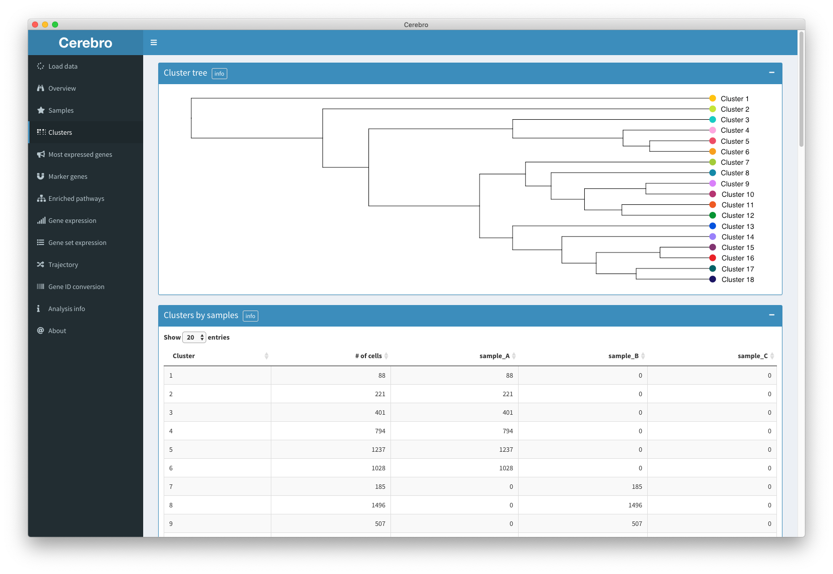
The “Clusters” panel gives a cluster-centric view of the data. Except for the first plot (the cluster tree), it shows the same info as the “Samples” panel however now the cells are grouped by the cluster they were assigned to.

The cluster tree shows you the similarity between clusters. This can be useful if you want to merge clusters and want to know which ones are most similar to each other.

Then, the composition of each cluster by sample is provided in the form of a table and plot, followed by distributions of the number of transcripts, expressed genes, and, if available, mitochondrial and ribosomal gene expression.

As before, we also see the distribution of clusters into the cell cycle phases from either Seurat or Cyclone, if they have been calculated.

Most expressed genes

The “Most expressed genes” panel provides tables with precisely the information promised by the title.

For each sample and cluster (select in the respective input box), you will see the 100 most expressed genes and what percentage of all transcripts they account for. Feel free to search the table through the search box, or download it in CSV or Excel format.

Marker genes

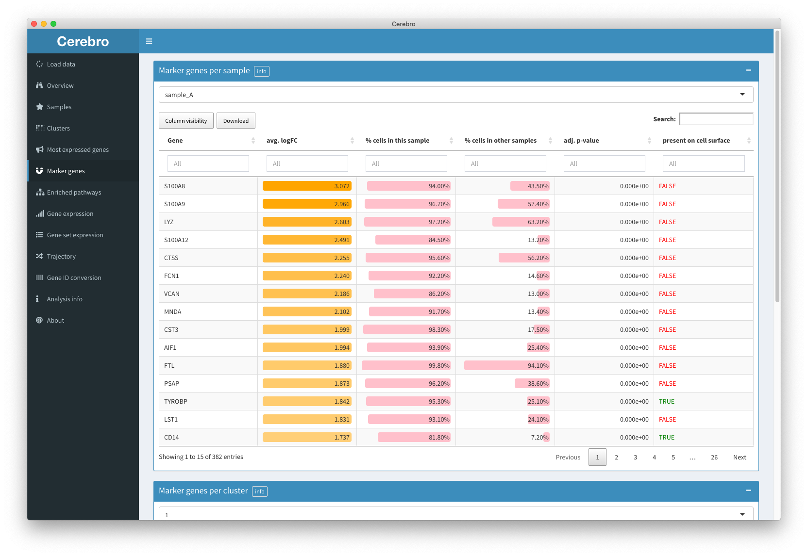
The “Marker genes” panel provides tables of - surprise - marker genes for each sample and cluster.

In the case of marker genes per sample, this list conceptually resembles differential expression analysis of a bulk RNA-seq experiment. Instead, the expression profiles of clusters are expected to be more homogeneous.

Marker genes should help to identify the cell type of a sample or cluster, and find new markers to purify that cell population.

It is important to know that in this analysis, each cell group (sample or cluster) is compared to all other cells combined. This is important because it means marker genes don’t have to be exclusive to one cell group. Instead, they can be shared by multiple groups.

There are multiple parameters and cut-offs that need to be chosen during the analysis. Check the “Marker genes” section in the “Analysis info” panel to find some details. You can sort the genes by the average logFC, the percentage of cells that express this gene (at least 1 transcript) in the cell population of interest or the rest of cells (which it is tested against), and the adjusted p-value. If analyzing human or mouse data, there will be an extra column indicating whether or not this gene might be present on the cell surface. This information is generated by checking if the genes are associated with the gene ontology (GO) term “cell surface” (GO:0009986). Even though this information is not 100% reliable, it might point you to genes which allow you to purify the respective cell population.

Enriched pathways

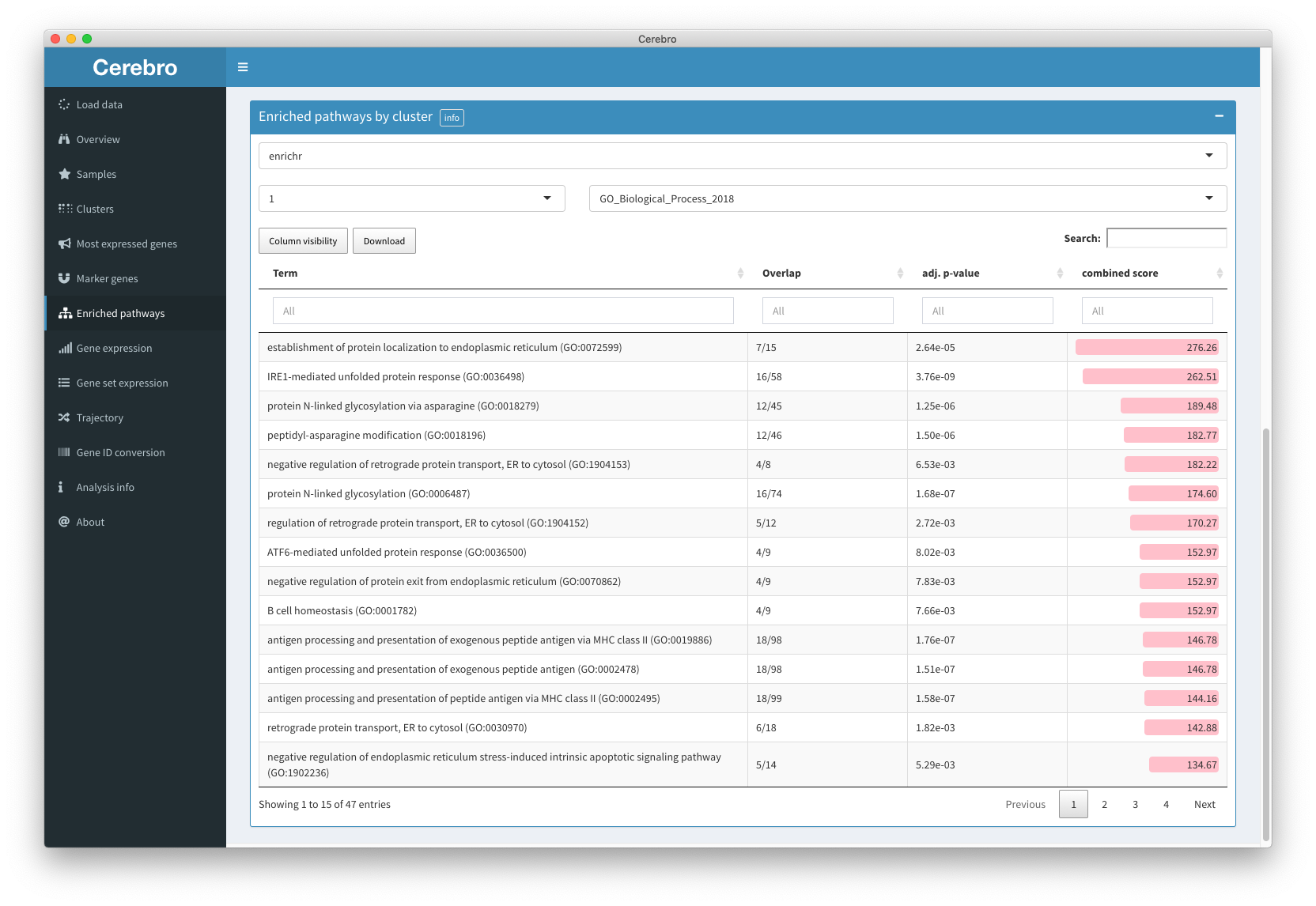
The “Enriched pathways” panel shows results of pathway enrichment analysis, again for each sample and cluster. There are currently two supported methods:

• Enrichr
• Gene Set Variation Analysis (GSVA)

Enrichr works by intersecting the marker genes of a sample/cluster with lists and data bases, such as gene ontology, KEGG, WikiPathways, and more.

GSVA, on the other hand, calculates the average expression of all genes for a given cell population (sample/cluster) and uses that to perform gene set enrichment analysis on a list of gene sets provided by the analyzing bioinformatician.

While both methods have the same goal of associating a cell population with functional (interpretable) terms, it is important to remember that Enrichr only uses the marker genes (their identification relies on other parameters) and GSVA uses all genes of the expression profile. Which of the two gives “better” results depends on the experimental context, which is why we support both methods.

Gene expression

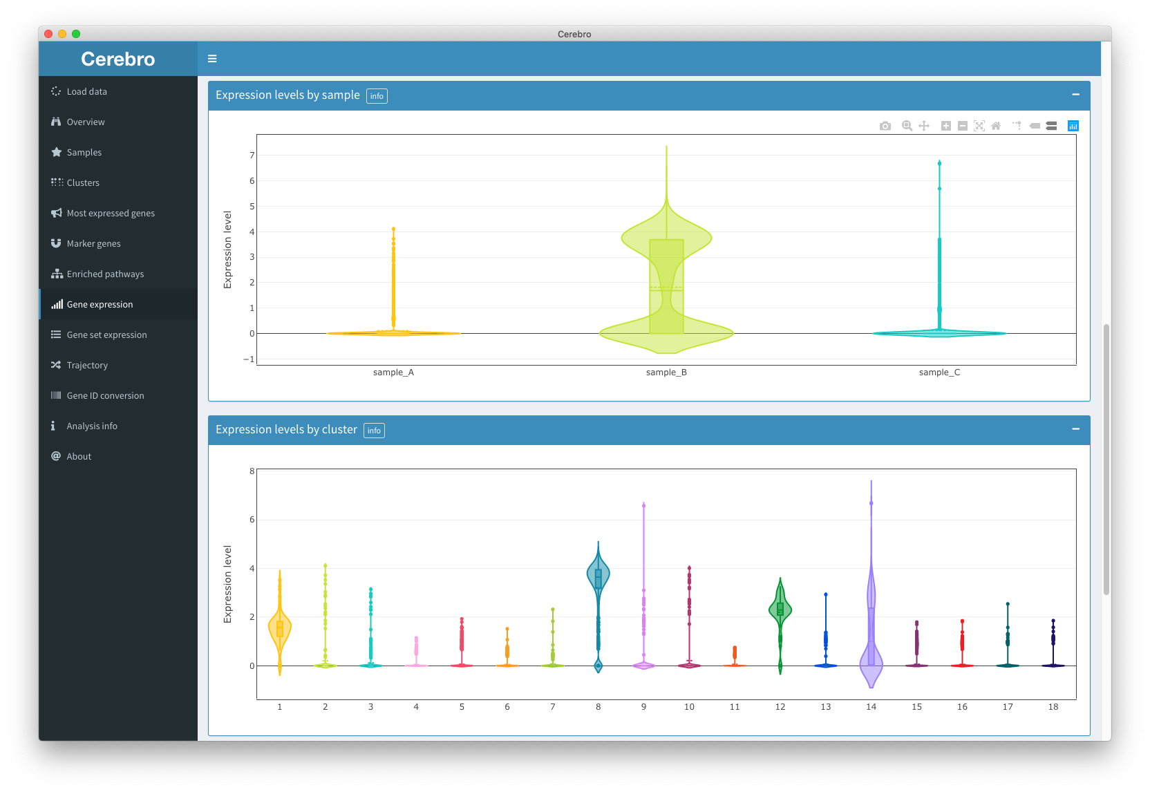
The “Gene expression” panel allows you to visualize the log-normalized expression of one or multiple genes.

The interface is similar to the one in the “Overview” panel. Cells are shown in the selected dimensional reduction, samples and clusters can be removed from the plot, and dot size size, opacity, as well as X and Y axis ranges can be adjusted. The color of each cell represents the expression of the queried genes (“Genes(s)” text box in top left corner). If inserting multiple genes, these must be posted on separate lines or separated through a comma (,), a space (), or semicolon (;). The colors are updated after you press ENTER or SPACE.

In addition to the dimensional reduction plot shown in the “Overview” panel, you may also choose whether cells should be plotted in random order or if you prefer to have cells with highest expression to be on top of the others.

Below the dimensional reduction you can see which genes are currently shown in the plot and which genes were not found (not present in the data set).

Further down you will find violin + box plots showing the distribution of expression of the selected genes grouped by sample and cluster.

The last plot of this panel shows the average expression of the 50 most expressed genes (of the ones specified by the user) across all cells to quickly spot which genes influence the color scale the most.

Gene set expression

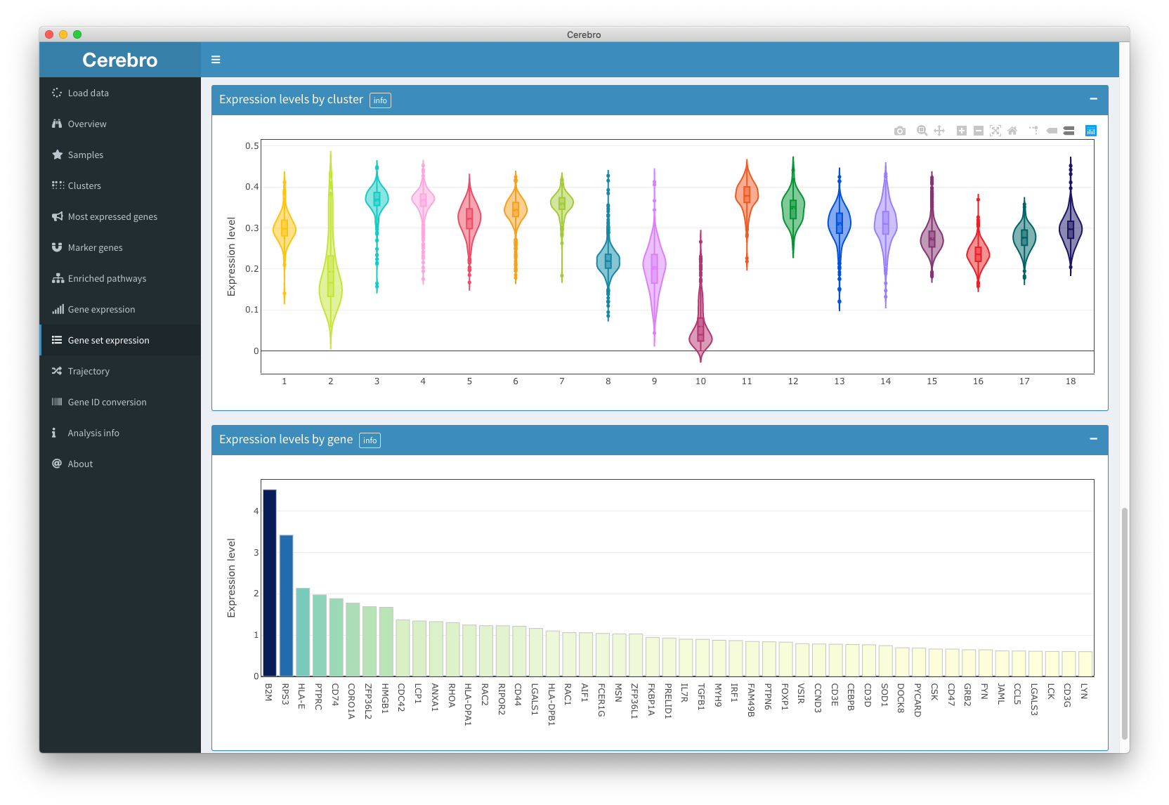
The “Gene set expression” panel is essentially the same as the “Gene expression” panel, except that it allows to select gene sets from MSigDB (requires internet connection). The MSigDB database is quite large, depending on your internet connection, it might take a few seconds to load the lists.

This feature is only available for human and mouse data.

Trajectory

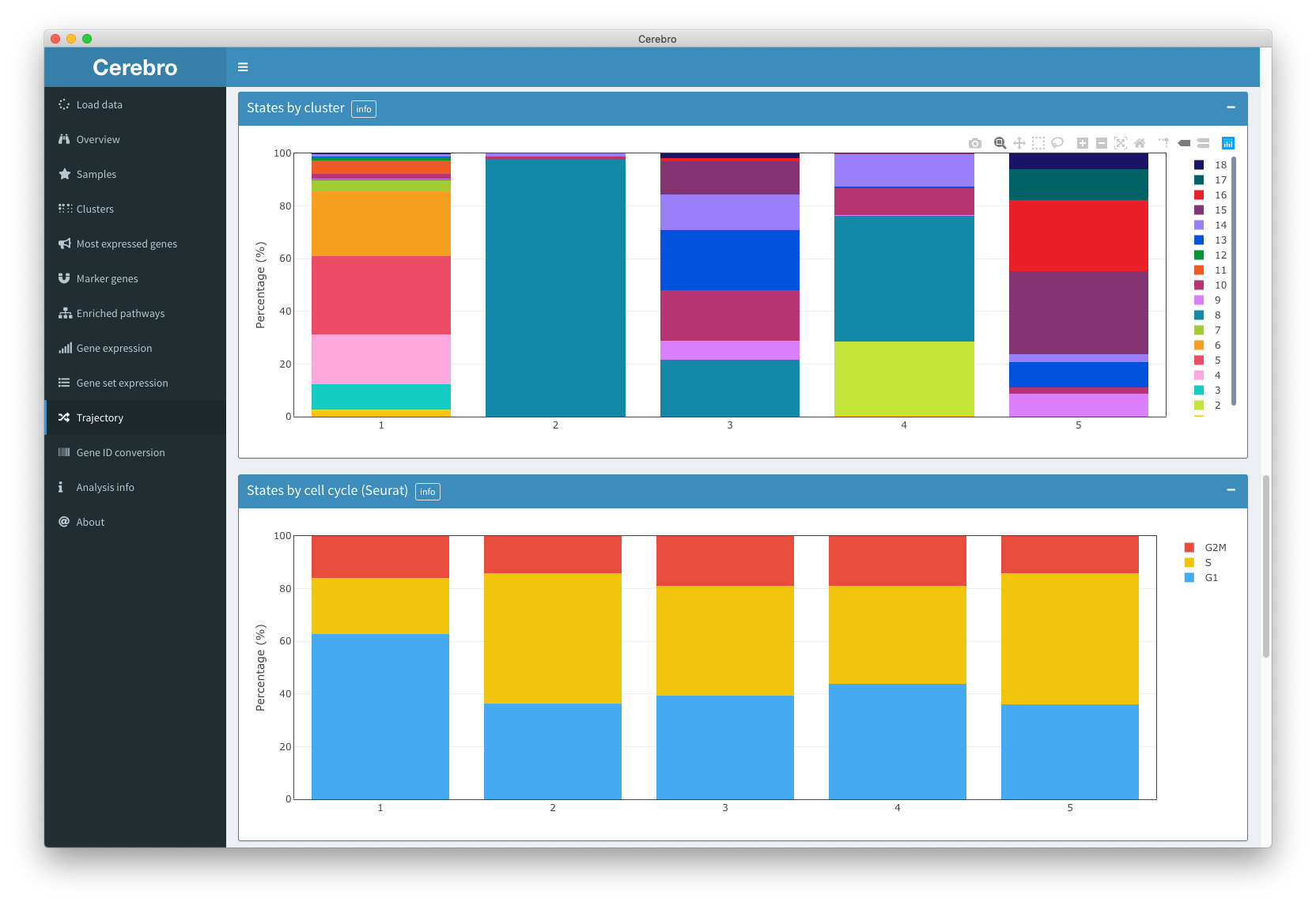
This “Trajectory” panel gives you access to trajectory information (if data is available).

Trajectories are another form of dimensional reduction which aim to preserve and highlight transitions within the data set.

Currently, we support trajectories generated by Monocle v2.

If multiple trajectories have been calculated, you can choose between them using the “Trajectory” field in the “Input parameters” box.

Similar to the other dimensional reduction plot we have discussed already, you can hide samples and clusters from the plot, and choose dot size and opacity. Cells can be colored by their transcriptional state (which is similar to the concept of a cluster, except that it is based on the calculated trajectory) and the pseudotime they were assigned (an approximation of how far along the transition a cell is), as well as all other available meta data (sample, cluster, number of transcripts, etc.). The black line represents the trajectory along which the cells are placed.

Below the dimensional reduction plot you can see the distribution of cells grouped by the meta data variable which is selected above over the calculated pseudotime.

Next, you have access to a table which tells you how many cells were found in each transcriptional state. If the meta data variable you selected at the top of the panel is a category, such as sample or cluster, each state will also tell you from which group those cells come.

The following plots are similar to what we have seen in the “Samples” and Clusters" panels. Namely, you see the composition of transcriptional states by sample, cluster and cell cycle, as well as their distribution of number of transcripts and expressed genes.

Gene ID conversion

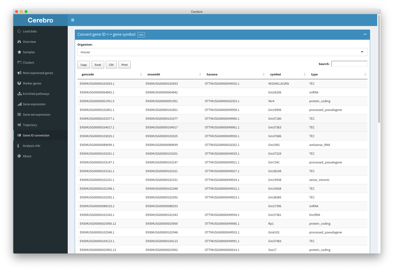
The “Gene ID conversion” panel provides tables which allow to convert gene IDs and names.

For the moment, only tables for mouse and human genes are available. The tables include GENCODE identifier, ENSEMBL identifier, HAVANA identifier, gene symbol and gene type and have been derived from the GENCODE annotation version M16 (mouse) and version 27 (human).

Analysis info

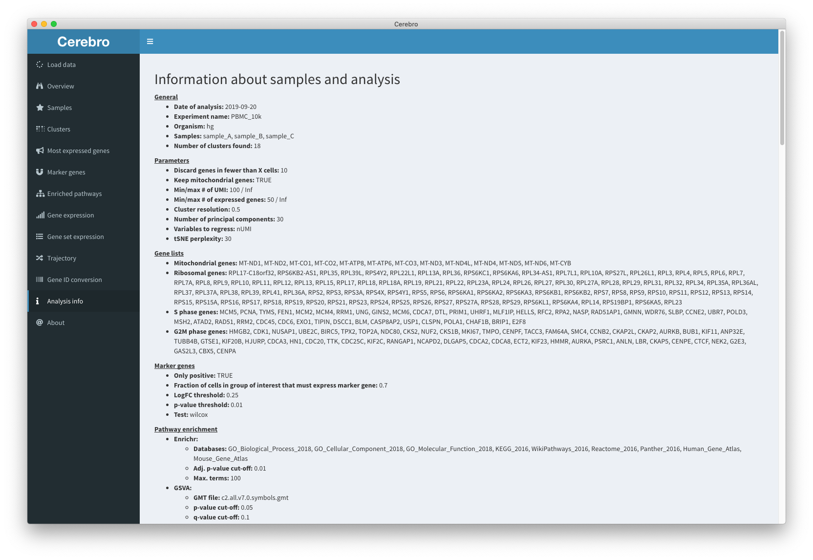
The “Analysis info” panel gives you an overview of the parameters which were used during the analysis (as long as they were recorded).

Shown can be:

• General information.
• Parameters used during pre-processing (cell/gene filtering, cluster resolution, etc.).
• Gene lists used for cell cycle analysis and calculation of the percentage of mitochondrial and ribosomal gene expression.
• Parameters used for marker gene detection.
• Parameters used for pathway enrichment analysis.
• Technical information.

About

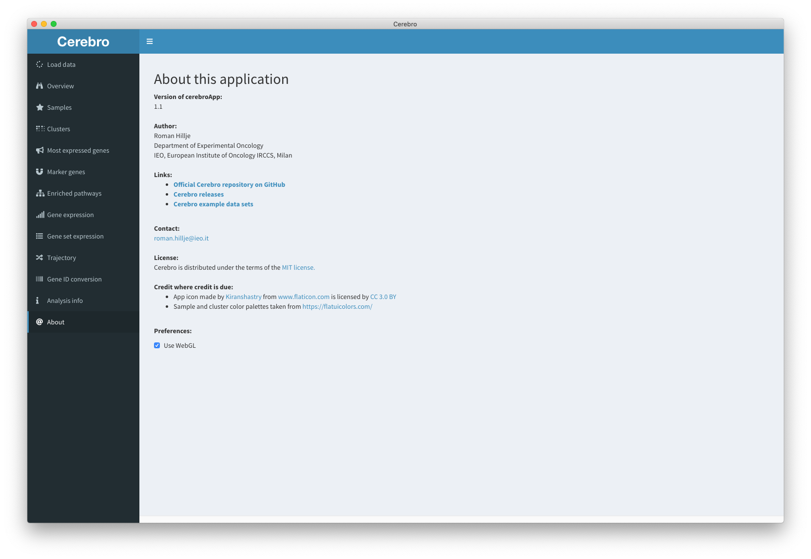
The “About” panel, apart from providing information about Cerebro and the author (me), allows to switch off WebGL (see “Preferences” at the bottom). Without going into detail, WebGL is a technology used to accelerate generation and interaction with complex graphics, such as the dimensional reduction plot with many cells. Most modern browsers should be compatible with WebGL, but if you experience problems with the dimensional reduction plots, for example cells/dots are not visible, switching off WebGL might fix that.

Addendum

Before letting you go to look at your data, I want to (briefly) address one question that you might have already asked yourself: Why should you Cerebro?

The aim of Cerebro is to facilitate the collaboration between experimental and computational biologists. There are is data exploration similar to Cerebro, however they usually fall into one of two categories:

• Made for computational biologists: That means these browsers are difficult to install and access, requiring the user to install packages and fiddle around with the terminal which is something that, at least from my experience, most experimental biologists are not experienced with.
• Made for experimental biologists: These browsers usually have great user interfaces but lock you (and the data) in their software making additional analysis starting from the same data set difficult (for the computational biologists).

We think Cerebro can bridge the gap by providing analytical flexibility and giving access to the data to those who aren’t involved in the analysis but have expertise to understand and interpret it.