Roman Hillje

Posts

Intensity plot 2

Jan 1, 0001

library(tidyverse)
library(viridis)

n <- 15000

data <- bind_rows(
  tibble(x = rnorm(n, 5, 2), y = rnorm(n, 7.5, 4)),
  tibble(x = rnorm(n, 10, 3), y = rnorm(n, 2.5, 3)),
  tibble(x = rnorm(n, 15, 4), y = rnorm(n, 10, 5))
)

p <- ggplot(data) +
  geom_hex(aes(x, y), bins = 50) +
  theme_bw() +
  labs(x = 'X', y = 'Y') +
  scale_fill_viridis(
    name = 'Count',
    guide = guide_colorbar(frame.colour = 'black', ticks.colour = 'black')
  ) +
  theme(legend.position = 'right')
ggsave('2.png', p, height = 5, width = 6)

Map of Trieste

Jan 1, 0001

Light version

library(sf)
library(foreign)
library(tidyverse)
library(lwgeom)
library(stringi)
options(stringsAsFactors = FALSE)

# download SHP files for region, e.g. from Geofabrik
# http://download.geofabrik.de/europe/italy/nord-est.html
buildings_a <- read_sf('gis_osm_buildings_a_free_1.shp')
landuse_a <- read_sf('gis_osm_landuse_a_free_1.shp')
natural <- read_sf('gis_osm_natural_free_1.shp')
natural_a <- read_sf('gis_osm_natural_a_free_1.shp')
railways <- read_sf('gis_osm_railways_free_1.shp')
roads <- read_sf('gis_osm_roads_free_1.shp')
traffic <- read_sf('gis_osm_traffic_free_1.shp')
traffic_a <- read_sf('gis_osm_traffic_a_free_1.shp')
transport <- read_sf('gis_osm_transport_free_1.shp')
transport_a <- read_sf('gis_osm_transport_a_free_1.shp')
water_a <- read_sf('gis_osm_water_a_free_1.shp')
waterways <- read_sf('gis_osm_waterways_free_1.shp')

# download the country boundaries as SHP file
# https://wambachers-osm.website/boundaries/
# we need it once with the border along the land area and once inside the water
# because the sea is not annotated in any of the other SHP files and if we draw
# the background blue, there will also be a blue border around the whole map.
# this trick is only possible because we have zoomed into the map far enough
# that all the parts of the sea seen in it still belong to Italy and therefore,
# when downloading the border of Italy including the water, we can use that to
# draw the sea and then the land on top
country_boundaries <- read_sf('country_boundaries/Italy_AL2.shp')
country_boundaries_with_water <- read_sf('country_boundaries_with_water/Italy_AL2.shp')

coordinates_box <- c(
  xmin = 13.738060,
  ymin = 45.620521,
  xmax = 13.804836,
  ymax = 45.670204
)

box <- list(
  coordinates = coordinates_box,
  buildings_a = st_crop(buildings_a, coordinates_box),
  landuse_a = st_crop(landuse_a, coordinates_box),
  natural = st_crop(natural, coordinates_box),
  natural_a = st_crop(natural_a, coordinates_box),
  railways = st_crop(railways, coordinates_box),
  roads = st_crop(roads, coordinates_box),
  traffic = st_crop(traffic, coordinates_box),
  traffic_a = st_crop(traffic_a, coordinates_box),
  transport = st_crop(transport, coordinates_box),
  transport_a = st_crop(transport_a, coordinates_box),
  water_a = st_crop(water_a, coordinates_box),
  waterways = st_crop(waterways, coordinates_box)
  country_boundaries = st_crop(country_boundaries, coordinates_box),
  country_boundaries_with_water = st_crop(country_boundaries_with_water, coordinates_box)
)

# makes it easier to come back to it later
saveRDS(box, 'box.rds')

blankbg <- theme(
  axis.line = element_blank(),
  axis.text.x = element_blank(),
  axis.text.y = element_blank(),
  axis.ticks = element_blank(),
  axis.title.x = element_blank(),
  axis.title.y = element_blank(),
  panel.background = element_blank(),
  panel.border = element_blank(),
  panel.grid.major = element_blank(),
  panel.grid.minor = element_blank(),
  plot.background = element_blank(),
)

p <-
  ggplot() +
  geom_sf(data = box$country_boundaries_with_water, color = 'black', size = 0.35, fill = '#78b1e4') +
  geom_sf(data = box$country_boundaries, color = 'black', size = 0.35, fill = 'white') +
  geom_sf(data = box$water_a %>% dplyr::filter(fclass %in% c('water')), size = 0, fill = '#78b1e4') +
  geom_sf(data = box$landuse_a %>% filter(fclass %in% c('grass','cemetery','forest','park')), size = 0, fill = '#65b8a2') +
  geom_sf(data = box$roads %>% dplyr::filter(fclass %in% c('unclassified','service','residential')), color = 'black', size = 0.15) +
  geom_sf(data = box$railways, size = 0.15, color = 'black') +
  geom_sf(data = box$roads %>% dplyr::filter(fclass %in% c('primary','primary_link','motorway','motorway_link','trunk','trunk_link')), color = 'black', size = 0.6) +
  geom_sf(data = box$roads %>% dplyr::filter(fclass %in% c('secondary','secondary_link')), color = 'black', size = 0.5) +
  geom_sf(data = box$roads %>% dplyr::filter(fclass %in% c('tertiary','tertiary_link')), color = 'black', size = 0.4) +
  geom_sf(data = box$buildings_a, color = '#7f8c8d', alpha = 0.5, size = 0.05, fill = '#7f8c8d') +
  blankbg +
  theme(plot.background = element_rect(fill = 'white', color = NA)) +
  coord_sf(xlim = box$coordinates[c(1,3)], ylim = box$coordinates[c(2,4)], expand = FALSE)

ggsave('trieste_light.png', p, scale = 1, width = 10, height = 10, units = 'in', dpi = 150)

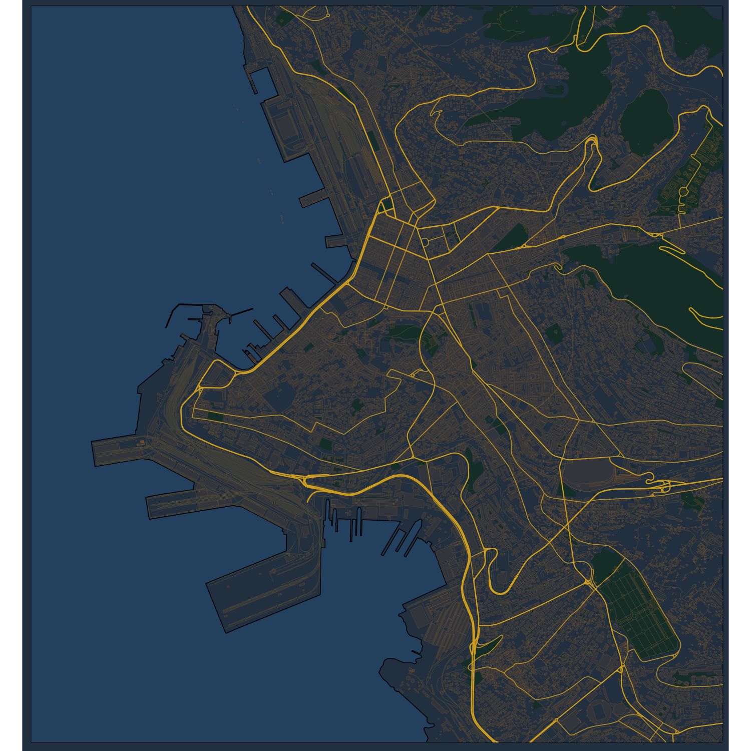
Dark version

library(sf)
library(foreign)
library(tidyverse)
library(lwgeom)
library(stringi)
options(stringsAsFactors = FALSE)

# load from previous code block
box <- readRDS('box.rds')

blankbg <- theme(
  axis.line = element_blank(),
  axis.text.x = element_blank(),
  axis.text.y = element_blank(),
  axis.ticks = element_blank(),
  axis.title.x = element_blank(),
  axis.title.y = element_blank(),
  panel.background = element_blank(),
  panel.border = element_blank(),
  panel.grid.major = element_blank(),
  panel.grid.minor = element_blank(),
  plot.background = element_blank(),
)

p <-
  ggplot() +
  geom_sf(data = box$country_boundaries_with_water, color = 'black', size = 0.35, fill = '#2d5272') +
  geom_sf(data = box$country_boundaries, color = 'black', size = 0.35, fill = '#2c3e50') +
  geom_sf(data = box$water_a %>% dplyr::filter(fclass %in% c('water')), size = 0, fill = '#2d5272') +
  geom_sf(data = box$landuse_a %>% filter(fclass %in% c('grass','cemetery','forest','park')), size = 0, fill = '#183b32') +
  geom_sf(data = box$roads %>% dplyr::filter(fclass %in% c('unclassified','service','residential')), color = '#6d5f43', size = 0.15) +
  geom_sf(data = box$railways, size = 0.15, color = '#6d5f43') +
  geom_sf(data = box$roads %>% dplyr::filter(fclass %in% c('tertiary','tertiary_link')), color = '#c39c30', size = 0.4) +
  geom_sf(data = box$roads %>% dplyr::filter(fclass %in% c('secondary','secondary_link')), color = '#d9ac25', size = 0.5) +
  geom_sf(data = box$roads %>% dplyr::filter(fclass %in% c('primary','primary_link','motorway','motorway_link','trunk','trunk_link')), color = '#d9ac25', size = 0.6) +
  geom_sf(data = box$buildings_a, color = '#cb862b', alpha = 0.25, size = 0.05, fill = '#7c5c3f') +
  blankbg +
  theme(plot.background = element_rect(fill = '#2c3e50', color = NA)) +
  coord_sf(xlim = box$coordinates[c(1,3)], ylim = box$coordinates[c(2,4)], expand = FALSE)

ggsave('trieste_dark.png', p, scale = 1, width = 10, height = 10, units = 'in', dpi = 150)

something went wrong... here should be a figure

Phylogenetic tree

Jan 1, 0001

library(tidyverse)
library(jcolors)
library(ggtree)

# load data
data(mtcars)

# choose number of carburetors as group
groups <- mtcars$carb %>% as.character() %>% unique() %>% sort()

# group data by carburetor and calculate means for all features
temp_data <- mtcars %>%
  group_by(carb) %>%
  summarise_all(list(mean = mean)) %>%
  as.matrix()
rownames(temp_data) <- groups

# calculate distance matrix
distance_matrix <- dist(temp_data)

# calculate phylogenetic tree
tree <- ape::as.phylo(hclust(distance_matrix))

# plot
p <- ggtree(tree, aes(x, y)) +
  scale_y_reverse() +
  geom_tree() +
  theme_tree() +
  geom_tiplab(label = paste0(tree$tip.label, ' carbs'), offset = 8) +
  geom_tippoint(color = jcolors('pal5'), shape = 16, size = 5) +
  coord_cartesian(clip = 'off') +
  theme(plot.margin = unit(c(0,1,0,0), 'cm'))
ggsave('phylogenetic_tree.png', p, height = 3, width = 4)

Scatter plot 1

Jan 1, 0001

library(tidyverse)

data(iris)

p <- iris %>%
  mutate(Petal.Width.larger = Petal.Width * 1.5) %>%
  ggplot() +
  geom_point(aes(Sepal.Length, Sepal.Width, size = Petal.Width.larger), color = 'black', show.legend = FALSE) +
  geom_point(aes(Sepal.Length, Sepal.Width, color = Petal.Length, size = Petal.Width)) +
  theme_bw() +
  labs(x = 'Sepal length', y = 'Sepal width', size = 'Petal width') +
  scale_color_distiller(
    palette = 'Spectral', name = 'Petal length',
    guide = guide_colorbar(frame.colour = 'black', ticks.colour = 'black')
  ) +
  theme(legend.position = 'right')

ggsave('1.png', p, height = 5, width = 6)

Scatter plot 2

Jan 1, 0001

library(tidyverse)
library(MASS)

# download differential expression data from EBI Expression Atlas database
# https://www.ebi.ac.uk/gxa/experiments/E-MTAB-7445/Results
t <- read_tsv('E-MTAB-7445-query-results.tsv', skip = 3) %>%
  rename(
    gene_id = 1,
    gene_name = 2,
    comparison_1_fold_change = 3,
    comparison_1_p_value = 4,
    comparison_2_fold_change = 5,
    comparison_2_p_value = 6
  )

# filter genes which have p-values lower than 0.1 im both comparisons
t_filtered <- t %>%
  filter(
    comparison_1_p_value <= 0.1,
    comparison_2_p_value <= 0.1
  )

# calculate density of dots as described on:
# https://slowkow.com/notes/ggplot2-color-by-density/
get_density <- function(x, y, ...) {
  dens <- MASS::kde2d(x, y, ...)
  ix <- findInterval(x, dens$x)
  iy <- findInterval(y, dens$y)
  ii <- cbind(ix, iy)
  return(dens$z[ii])
}

t_filtered$density <- get_density(
  t_filtered$comparison_1_fold_change,
  t_filtered$comparison_2_fold_change,
  n = 100
)

# build color palette on https://gka.github.io/palettes
colors <- c('#7ac6e7', '#6badd9', '#5c95cb', '#4e7ebd', '#3f66af', '#314fa2',
  '#223894', '#132086', '#000275')

p <- t_filtered %>%
  arrange(density) %>%
  ggplot() +
  geom_point(
    aes(comparison_1_fold_change, comparison_2_fold_change, color = density),
    size = 4, show.legend = FALSE
  ) +
  geom_hline(yintercept = 0, linetype = 'dashed') +
  geom_vline(xintercept = 0, linetype = 'dashed') +
  theme_bw() +
  labs(x = 'logFC - comparison A', y = 'logFC - comparison B') +
  scale_color_gradientn(colors = colors)
ggsave('2.png', p, scale = 1, height = 5, width = 6)

Scatter plot 3

Jan 1, 0001

library(tidyverse)
library(Seurat)

# create color palette from flatuicolors.com
colors_dutch <- c(
  '#FFC312','#C4E538','#12CBC4','#FDA7DF','#ED4C67',
  '#F79F1F','#A3CB38','#1289A7','#D980FA','#B53471',
  '#EE5A24','#009432','#0652DD','#9980FA','#833471',
  '#EA2027','#006266','#1B1464','#5758BB','#6F1E51'
)
colors_spanish <- c(
  '#40407a','#706fd3','#f7f1e3','#34ace0','#33d9b2',
  '#2c2c54','#474787','#aaa69d','#227093','#218c74',
  '#ff5252','#ff793f','#d1ccc0','#ffb142','#ffda79',
  '#b33939','#cd6133','#84817a','#cc8e35','#ccae62'
)
custom_colors <- c(colors_dutch, colors_spanish)

# load a single cell expression data set (generated in the lab I work at)
seurat <- readRDS('seurat.rds')

# calculate center position for each cluster
UMAP_centers_cluster <- tibble(
    UMAP_1 = as.data.frame(seurat@reductions$UMAP@cell.embeddings)$UMAP_1,
    UMAP_2 = as.data.frame(seurat@reductions$UMAP@cell.embeddings)$UMAP_2,
    cluster = seurat@meta.data$seurat_clusters
  ) %>%
  group_by(cluster) %>%
  summarize(x = median(UMAP_1), y = median(UMAP_2))

# plot
p <- bind_cols(seurat@meta.data, as.data.frame(seurat@reductions$UMAP@cell.embeddings)) %>%
  ggplot(aes(UMAP_1, UMAP_2, color = seurat_clusters)) +
  geom_point(size = 0.2) +
  geom_label(
    data = UMAP_centers_cluster,
    mapping = aes(x, y, label = cluster),
    size = 4.5,
    fill = 'white',
    color = 'black',
    fontface = 'bold',
    alpha = 0.5,
    show.legend = FALSE
  ) +
  theme_bw() +
  scale_color_manual(values = custom_colors) +
  labs(color = 'Cluster') +
  coord_fixed() +
  guides(colour = guide_legend(ncol = 1, override.aes = list(size = 2))) +
  theme(legend.position = 'right')
ggsave('3.png', p, height = 7, width = 7)